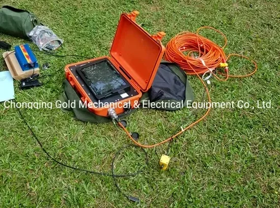
ASCE 7 Chapter 20 and the IBC mandate site-specific shear wave velocity data for Seismic Site Class determination, and in Corpus Christi the subsurface is rarely a textbook case. The transition from Holocene barrier island sands to the Beaumont Formation’s stiff clays happens abruptly across the city, creating velocity contrasts that boreholes alone miss. We run P-wave and S-wave seismic tomography lines — both refraction and reflection — to map these transitions directly, delivering 2D velocity cross-sections that feed into foundation design, liquefaction screening, and seismic hazard analysis. Our field spreads use 24- to 48-channel seismographs with vertical and horizontal geophones, processing in SeisImager and Rayfract to invert travel-time data into layered velocity profiles. For deep excavations near the ship channel or heavy structures on Padre Island Drive, CPT testing complements the velocity model with continuous tip resistance and pore pressure data, tying geophysical boundaries to geotechnical engineering properties without interpolation.
A buried paleochannel with 40% lower shear wave velocity can shift a site from Site Class D to E — and it won't show up on a standard boring log.
Local geotechnical context
The most common mistake we see in Corpus Christi is relying on N-value correlations alone to estimate shear wave velocity for Site Class determination. Oftentimes the local Beaumont clay is overconsolidated from desiccation, and its VS is 30-50% higher than what a generic SPT-VS correlation predicts — meaning a site gets misclassified as Class E when it's actually Class D, triggering unnecessary seismic detailing costs. The reverse also happens: loose fluvial sands beneath a stiff surface crust yield low VS that borings don't flag because SPT blow counts look acceptable in the upper 20 feet. Seismic tomography measures wave propagation directly; it doesn't infer velocity from penetration resistance. The ASTM D5777 standard specifies straight-ray and curved-ray inversion methods, and we run both, checking for hidden-layer problems that plague simple refraction interpretation. A velocity model also feeds directly into site-specific response analysis per ASCE 7 Section 21, which can justify reduction factors that code-default approaches cannot.
Questions and answers
How much does a seismic tomography survey cost in Corpus Christi?
How does seismic tomography differ from MASW in site classification?
MASW measures surface-wave dispersion to produce a 1D VS profile beneath the array center — it's fast and works well for layered sites. Seismic refraction tomography produces a true 2D cross-section from body waves, so it resolves lateral velocity changes — like channel fills, faults, or dipping bedrock — that a 1D MASW curve averages out. We often run both on the same spread and jointly invert the data for the most solid velocity model.
What depth can seismic refraction tomography reach in Corpus Christi soils?
Refraction depth depends on spread length and source energy. With a 240-foot spread and a weight-drop source, we typically image to 60-80 feet in the unconsolidated sands and clays common around Corpus Christi. Reflection surveys, using higher fold and CMP stacking, can reach 200 to 300 feet — enough to map the contact between Quaternary sediments and the underlying Tertiary formations. We design the acquisition geometry to meet your specific depth target.
Do I need seismic tomography if I already have SPT borings on my site?
Borings give you point data on soil type and penetration resistance. But for Site Class determination under IBC, you need shear wave velocity measured directly — not inferred from N-values. Seismic tomography provides continuous VS data between boreholes, catches lateral anomalies that borings miss, and can often justify a more favorable Site Class than default correlations would allow. It is the difference between assuming and knowing your site's seismic response.